Last time we left off with the general understanding of what GPT is and how information enters the model.
In this post we’ll go over what happens inside it, detailing the seemingly ever-present attention mechanism. I’ll start with explaining concepts using intuitive ideas, gradually building up to an understanding of attention mechanically.
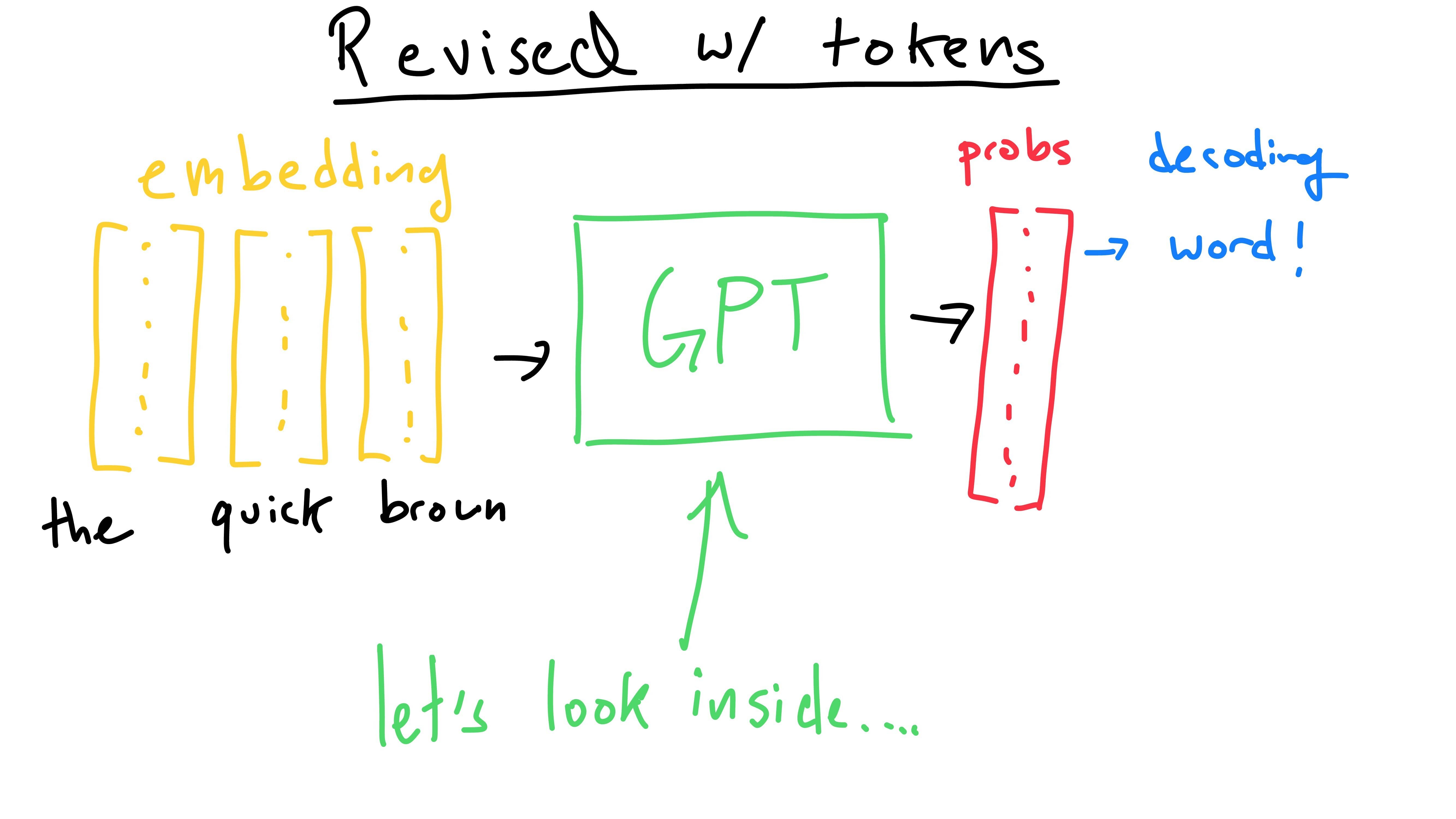
Here we can view the token embeddings (we know what these are!) entering the model and output probabilities exiting it. Let’s take a peek inside the box.
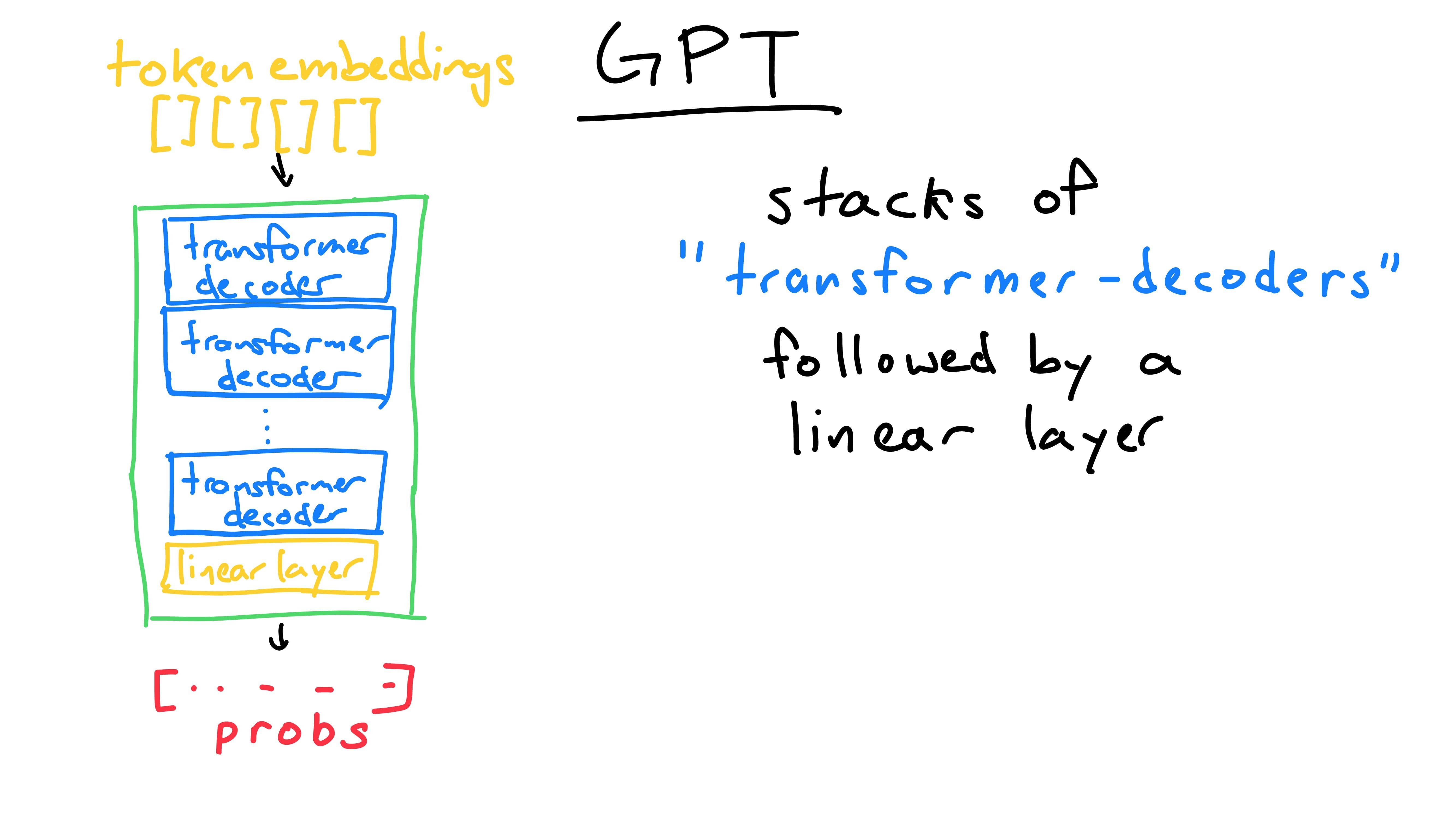
The internals of a GPT model are relatively simple - repeated “transformer decoder” blocks, finally followed by a linear layer. The linear layer is self-explanatory and we can look at it later. For now, let’s examine one of these mystical “transformer decoder” blocks.
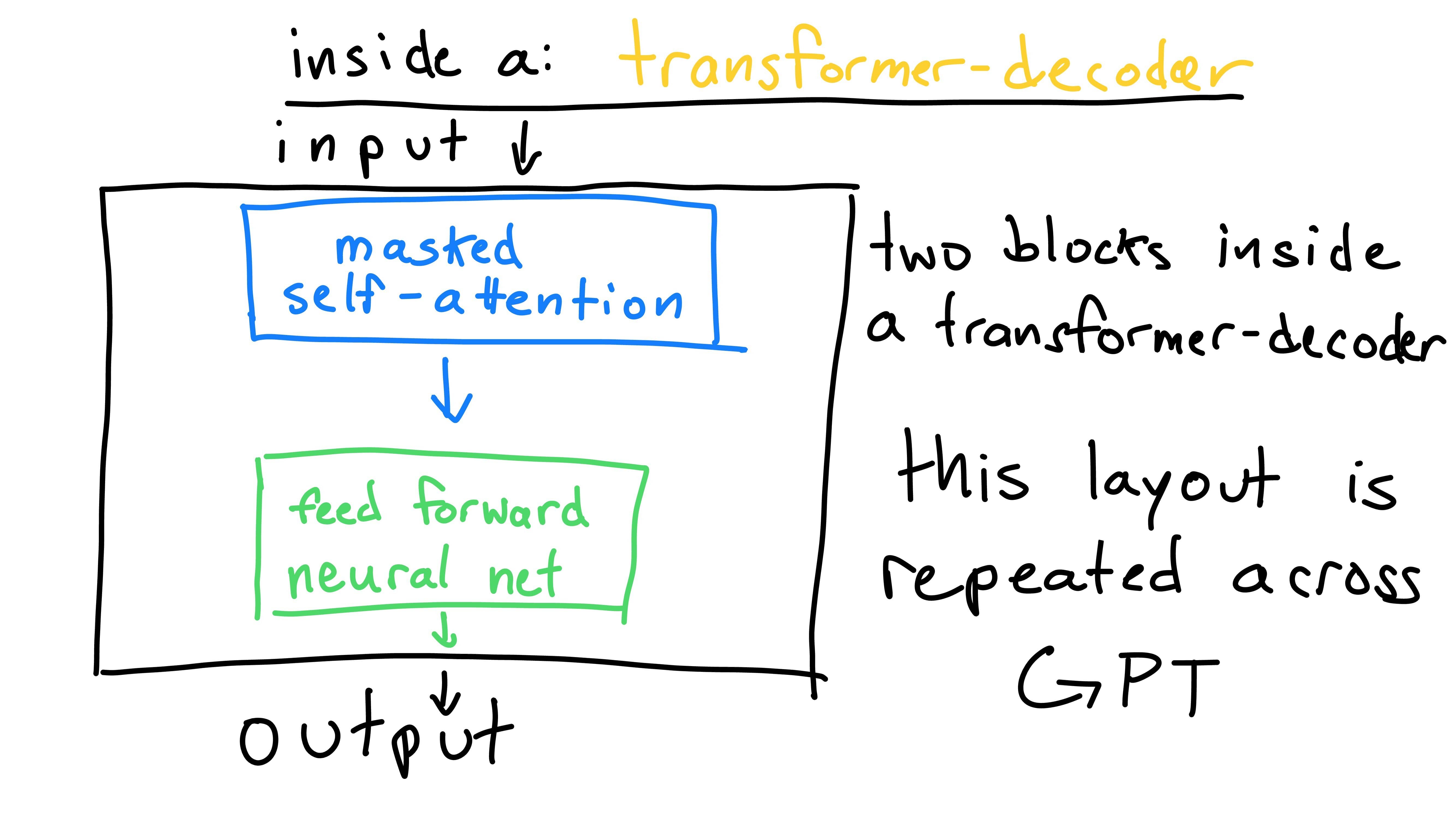
The block is comprised of two parts: masked self-attention, and a linear layer (feed forward neural network). Each block has the same structure (or architecture), but will contain different valued weights. For now, let’s only consider the “masked self-attention” in a conceptual manner. We’ll bring it back to implementation in a moment.
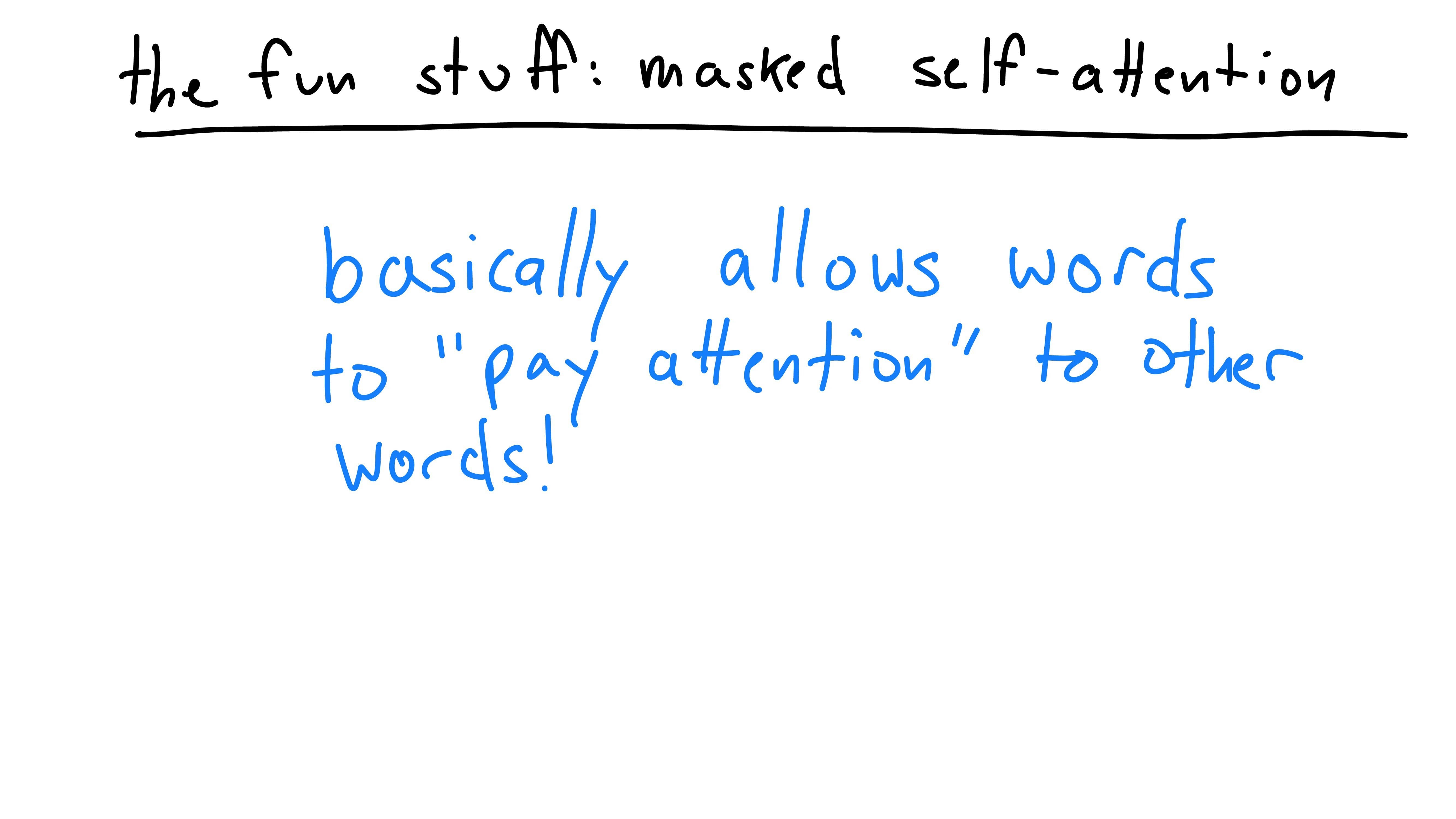
Masked self-attention is the mechanism that allows other words to pay attention to each other (and themselves), hence the “self-attention.” Words seldom exist alone and context determines what a word’s meaning is. To know the meaning of a word, one must also look at the words around it.
Here’s an example:
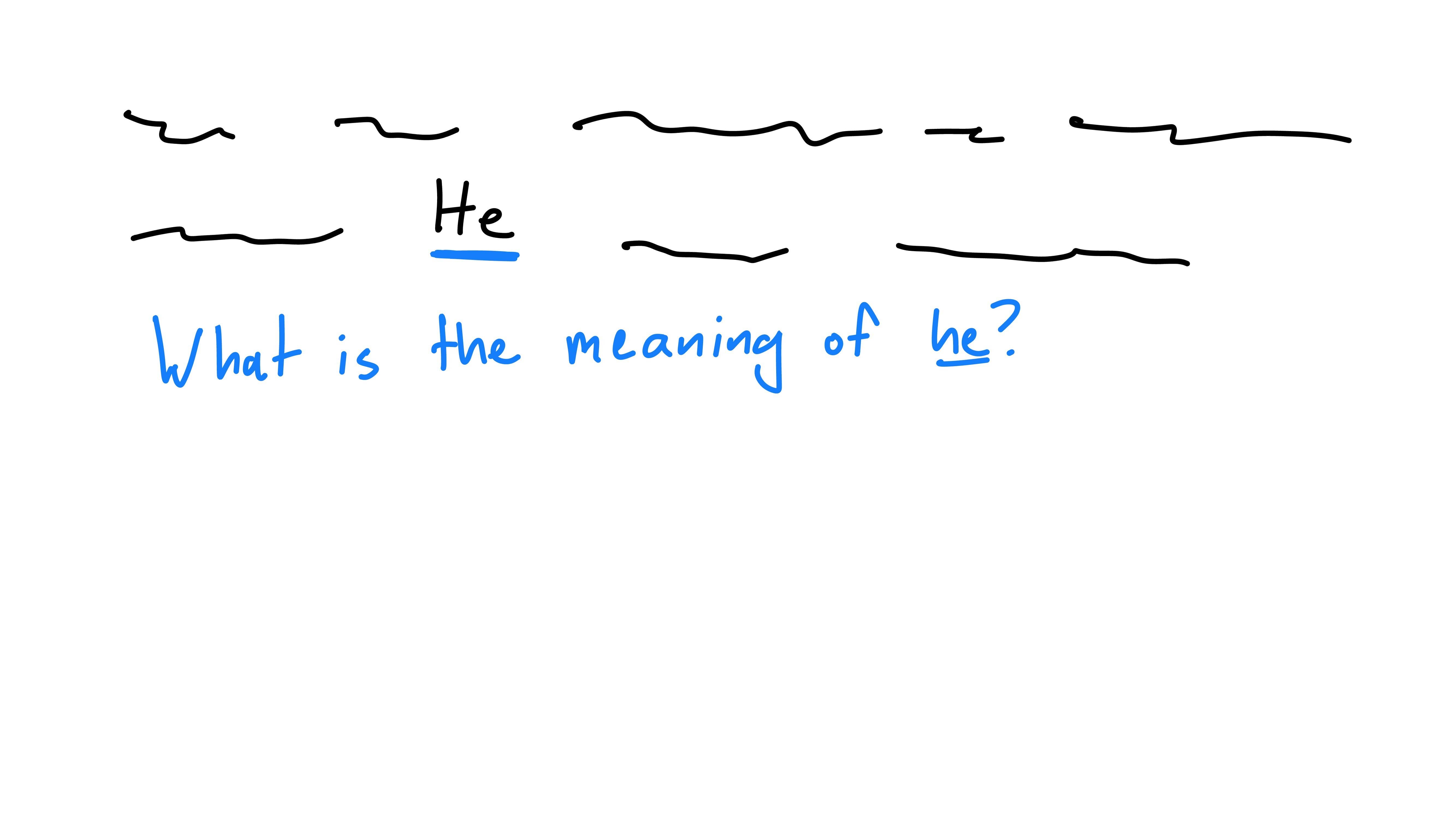
Here’s a phrase with all other words blanked out, besides the word “He”. If I asked you to explain what “He” represents, you’d likely look at me dumbfounded. Without gleaning context from other words, its impossible to figure out what “He” means!
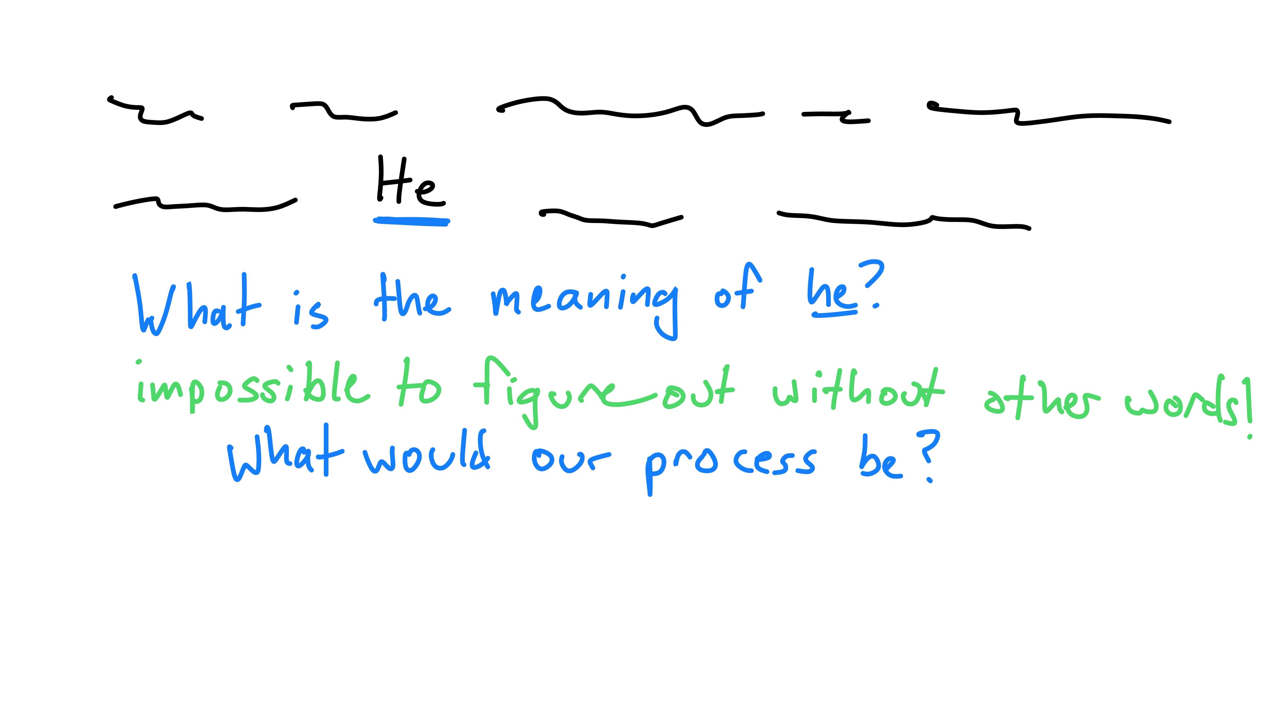
I raise this example to demonstrate that we need to do something to figure out the meaning of “He”. I’ll suggest a process that’s reasonable.
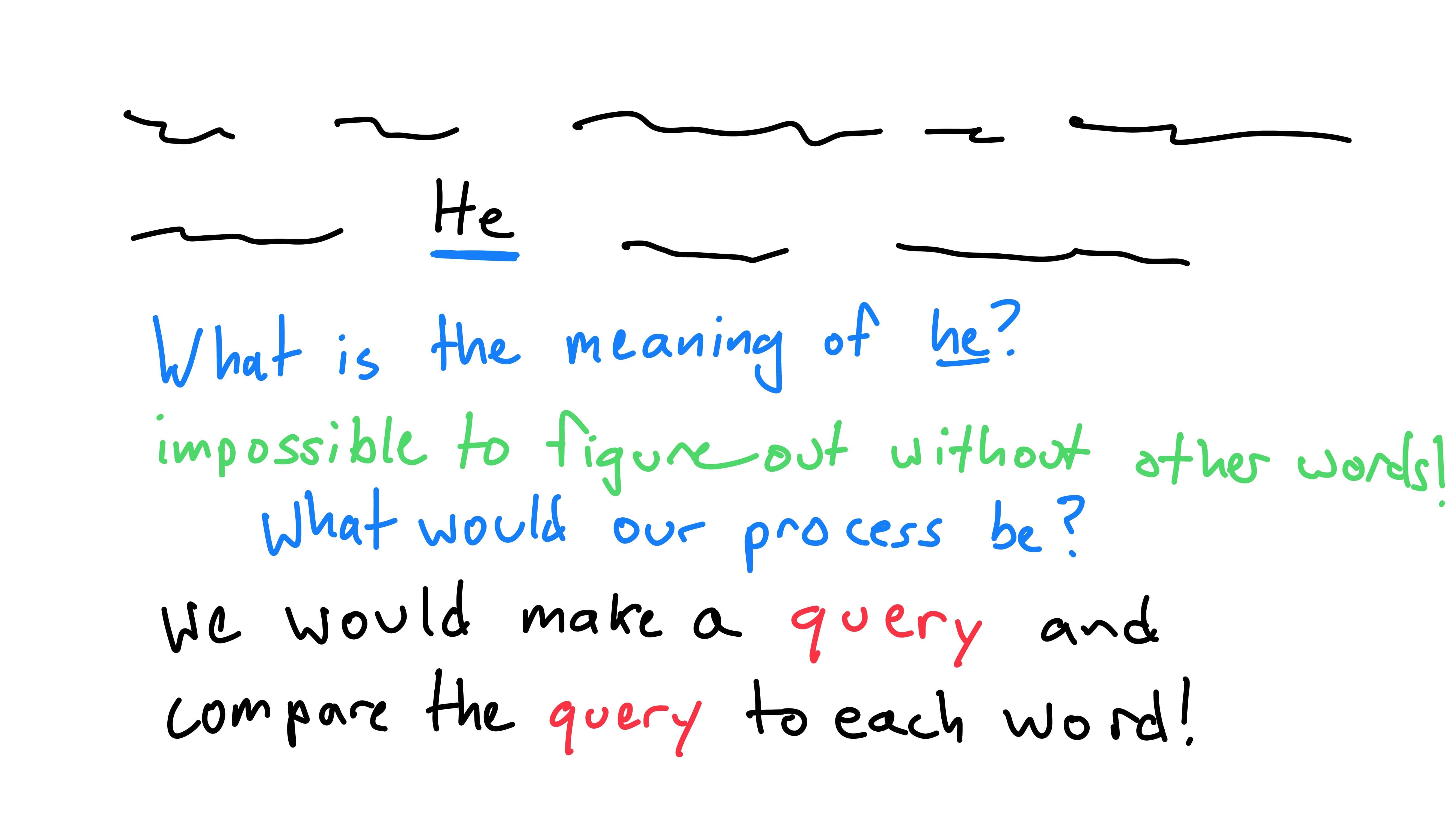
First off, we’d need to know what we’re even looking for, some sort of query. This query could be compared to words to see if they’re correlated.
At this point, I’ll have to reveal the secret sentence… (thank you I2 for listening to me!)
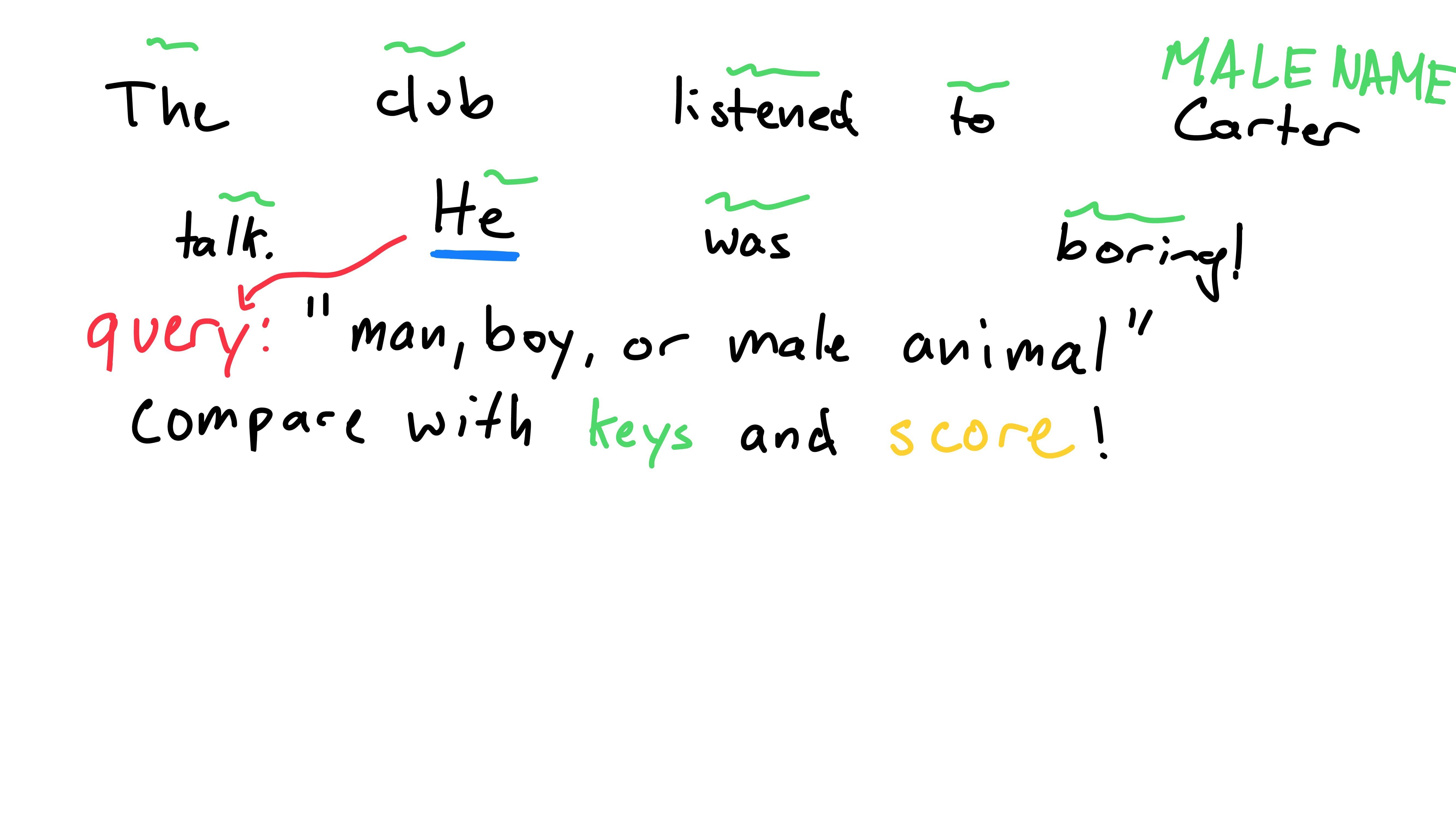
Jokes aside, we need a query for the word “He” (note: this is the query for “He”, not “He” getting queried). “He” refers to a “man, boy, or male animal”, so that seems like a good query!
Now, I’ll hit you with the most difficult part. We don’t want to compare the query directly to other words. Instead, we want to compare the query to a word’s identifiers or tags. I’ll give you an example for the word “Carter”:
When comparing “Carter” and the query “man, boy, or male animal”, we don’t actually find the similarity between the word “Carter” and the query. Instead, we compare the similarity of Carter’s identifiers! There are many ways to identify me: human, male, speaking, etc. This identifier is a key for “Carter”. Words need these keys to compare to queries, rather than just the word itself.
We give each word a key, an identifier to what it represents. These then allow us to compare the query to each word’s key, resulting in a similarity score for each word (with respect to the original word “He”).
Now that we have similarity scores for how much “He” is influenced by words (including itself), we just have to figure out what that means - quite literally. We give each word a value, what the word represents. The difference between a word itself and its value is less clear-cut with examples. One can think of it as what a word could mean to other words, not necessarily its true self. Finally, the meaning of “He” could be found by combining all of the values with respect to their scores (eg. “Carter” has a high score, so his value would influence the outcome of “He” more than “was”, which has a low score).
To figure out the meaning of any other word we could do the same process. Create a query for the word we are trying to find the meaning of, compare the query to each word’s key, resulting in a score. Then, combine each word’s value with respect to the word’s score to get the meaning!
(Note: this is difficult and this real-world explanation might not make sense. If so, I’d recommend reading Jay Alammar’s excellent analogy using manila folders and values.)
Guess what? We can do the same thing using a whole lot of vectors! For the moment, ignore how the vectors are created! We’ll get to that soon!
Translated into vector-land, we first create a query, key, and value vector for each word. To find the representation (or transformation) of one word, we use that word’s query.
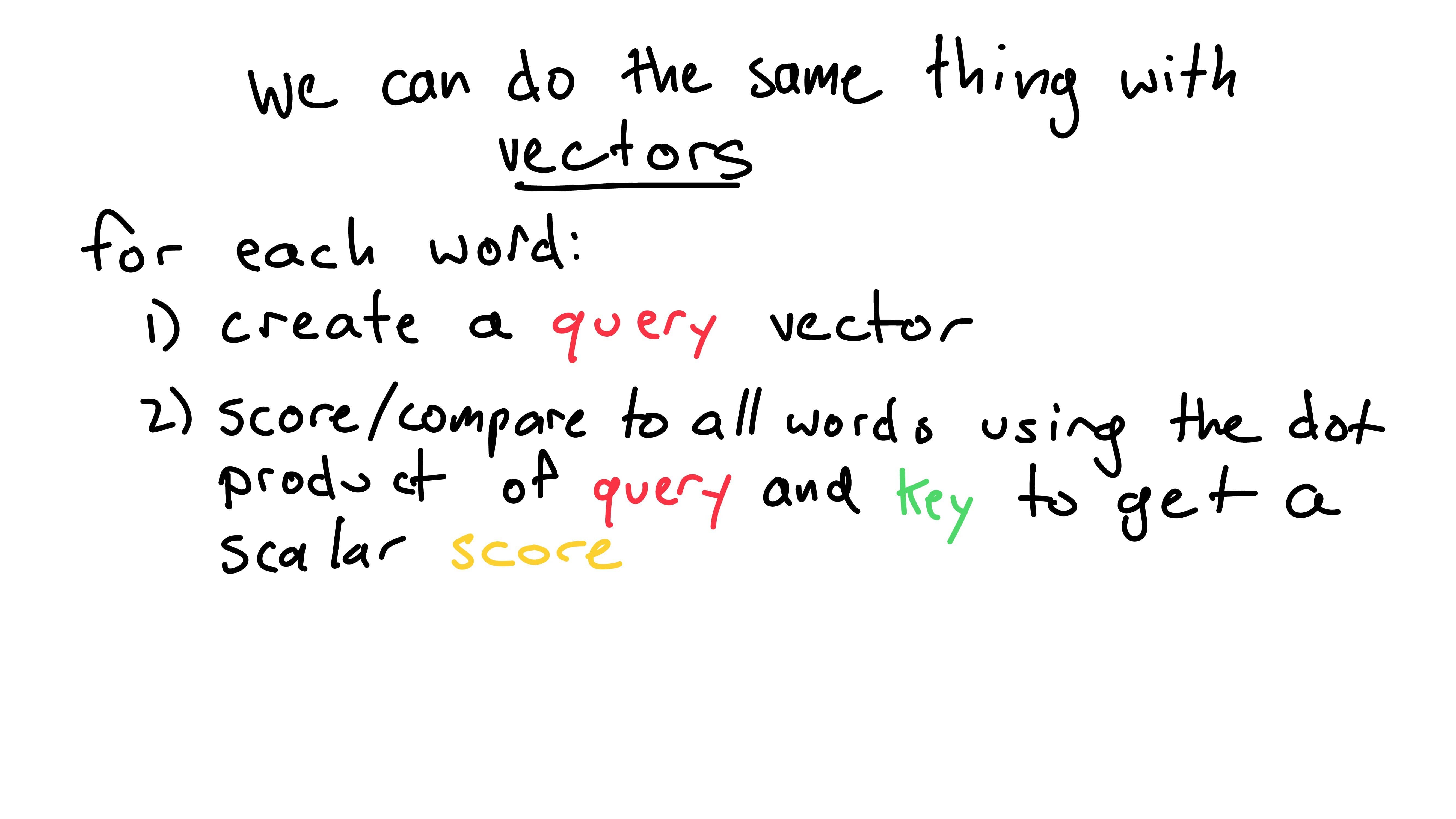
The scalar similarity score for a word is the result of the dot product of the word’s key vector and the query vector. This gives us a score for each word.
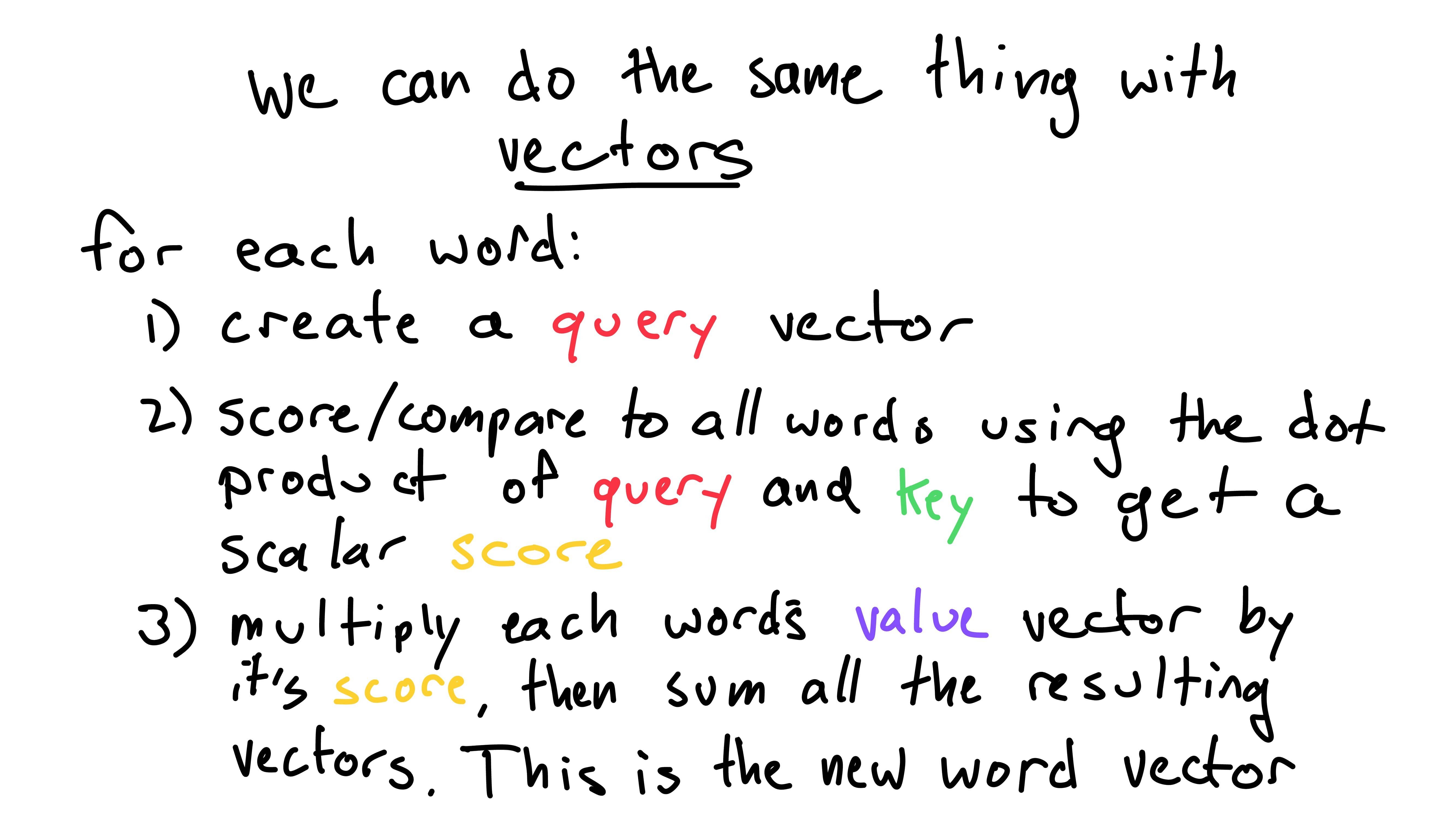
We then normalize the scores such that they sum to one (softmax). Finally, we multiply each word’s value vector by its respective score. Sum these results and we are left with the transformed word!
Let’s return to the important detail we glossed over - how are these vectors created?
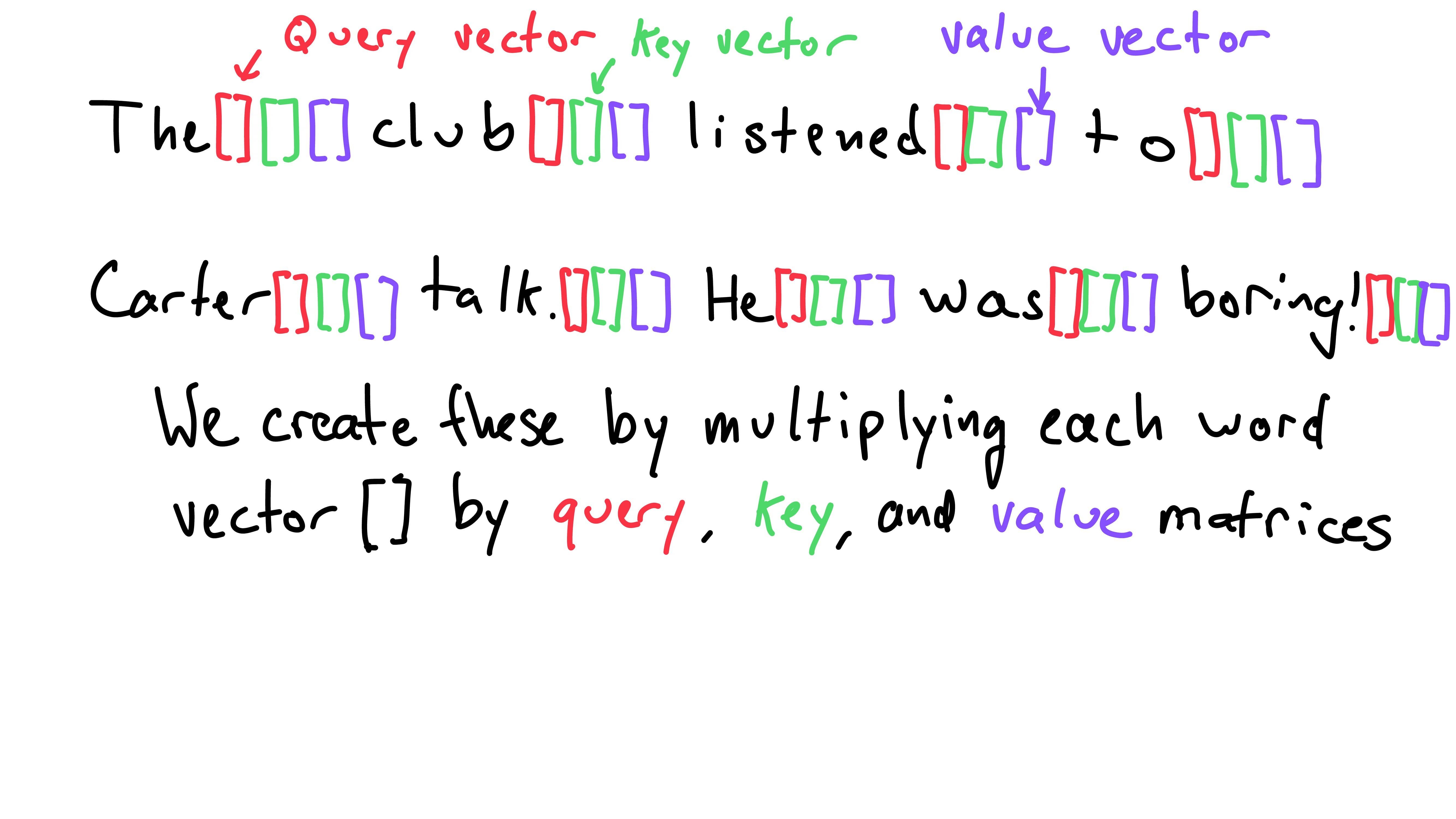
We use key, value, and query weight matrices to create an individual
key, value, and query vector for each word. These key, value, and query
vectors are of length d_key. I’ll get to how the size
d_key is found in a minute - for now we can assume it is
the same length as d_model. As word vectors throughout the
model are of size d_model, the weight matrices dimensions
are: (d_model, d_key).
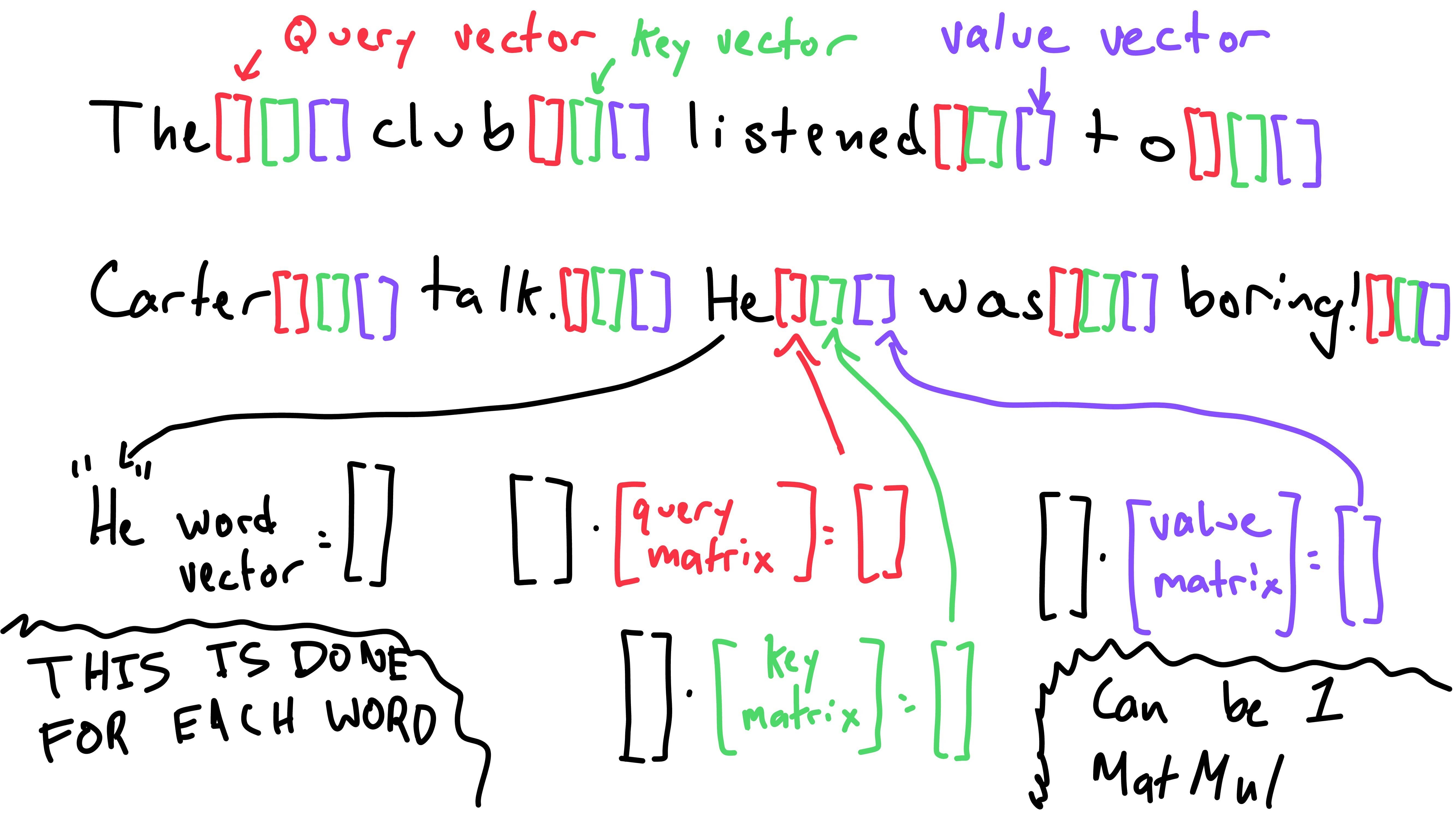
Thus, when we matrix multiply a word vector by a weight matrix, we
result in a vector of size d_key. We create these query,
key, and value vectors for each word vector.
Then, we need to score all words in relation to a query. Note that we will compare all words to all queries - I’m walking through comparing all words to only one query for demonstrations sake. The query for “He” has to be compared to all words, as does the query for “The”, “club”, and so on.
To score all words keys in relation to one query, we take the dot product of a word’s key and the query to obtain a scalar score. Note that we are still using one query - “He”s in the example below - to compare to all word’s keys.
Eg. the score for the word “club” in relation to “He”s query is the dot product of the the key for “club” and the query for “He”.
To normalize all the scores, we take the softmax of them. This just compresses each score between 0 and 1, while ensuring they all sum to 1. (Read more about the softmax function here)
We’re almost there! Next, we multiply each word’s value vector by its respective score. We can think of this step as weighting each word’s value vector by how much it is related/matters, its scalar score.
Finally, we sum all of the weighted value vectors, into one final
vector of length d_key. As I mentioned, we should currently
assume d_key is the same as d_model. Thus, we
have transformed the original “He” vector into a new one! We
would do this for each query, transforming each word.
There are some things that I’ve skipped over, but we’ve gotten past the hard part! Congrats!
These previous operations can be efficiently and compactly using tensors and matrix multiplication.
We can represent the input to the masked self-attention layer as a
tensor (higher dimensional matrix) with shape:
(batch_size, sequence_len, d_model).
batch_size is the number of sequences (sentences/phrases)
in the batch. (If you don’t know what a “batch” is, we group multiple
sequences for efficiency. You can read about it here).
sequence_len is the length of the sequence or sentence (the
largest length in the batch - we would need to pad other sequences to
the same length). We already know what d_model is! We get
this tensor by making the word vectors in a sequence just one matrix
(stacking all of the vectors together).
After passing this input through the masked self-attention, the
output will have the same shape:
(batch_size, sequence_len, d_model).
We’re going to ignore the batch dimension for this walk-through, as it stays constant throughout. Let’s take a peek at how queries, keys, and values are created.
Instead of having individual query, key, and value vectors for each
word, we have a query, key, and value matrix for the sequence. In the
above slide, I used T instead of sequence_len
and dk instead of d_key. They’re the same
thing.
Taking the matrix multiplication of the input matrix,
(T, d_model), and the query weight matrix,
(d_model, dk), we result in a query matrix of shape
(T, dk). Note that this is the same as using individual
vectors - here the vectors are stacked on top of each other. The key
vector for the second word would be the second row of the key matrix, so
on for other words/matrices.
Here we can see the generated query, key, and value matrices - all with the same shape.
If we recall back before matrix-land, the next step in pseudocode roughly is:
for query in query:
    for word in words:
        # score word to query using dot product
        word's score for the query = word's key (dot product) query
If we wanted to take the score for the i'th word’s key
with respect to the j'th word’s query, we would take the
dot product of the two. This can still be done using the query and key
matrices. All we need to do is take the dot product of the
i'th row in the keys matrix and the
j'th row in the queries matrix.
We could do this for each queries row, with regards to
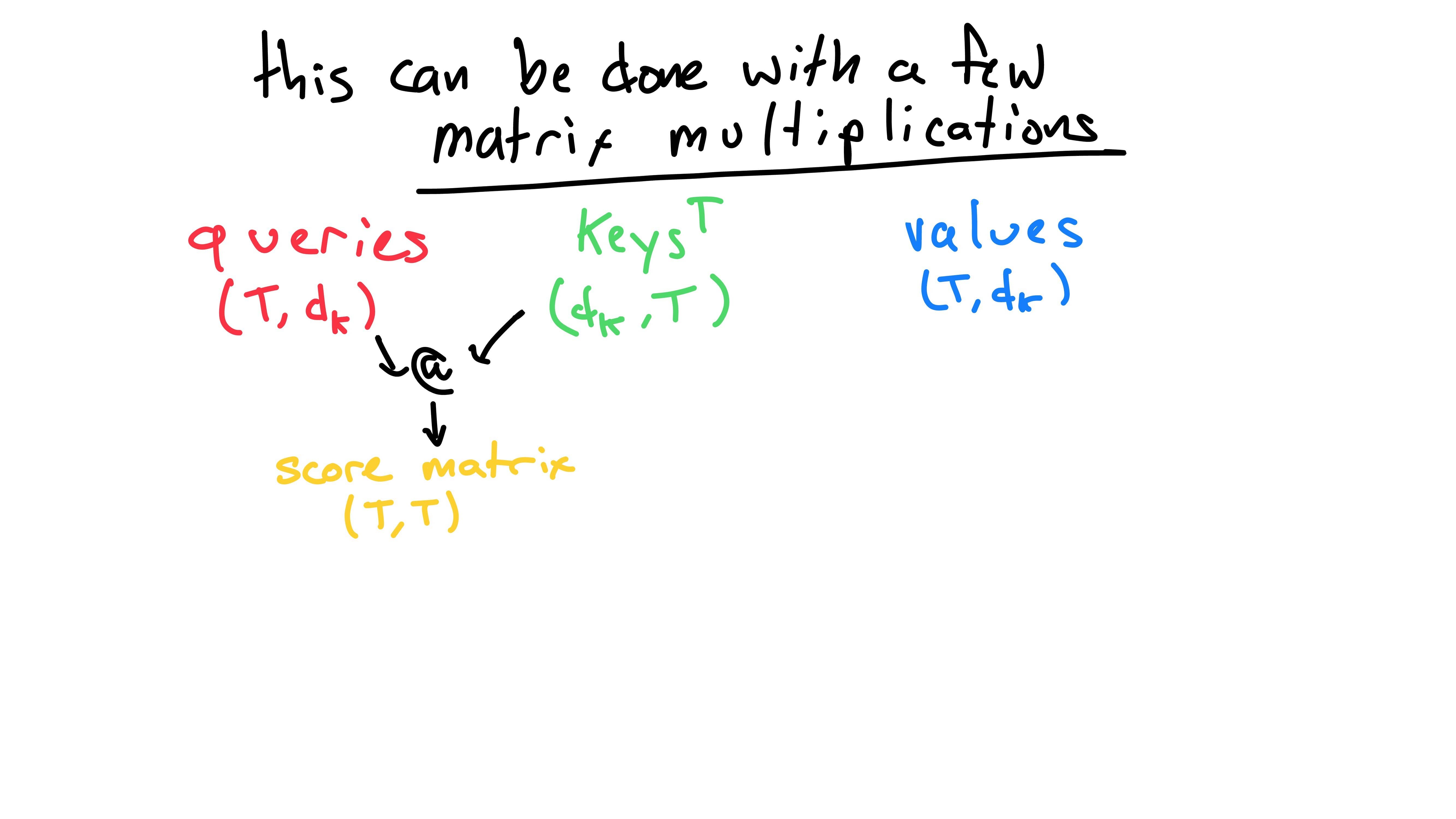
each keys row. However, there’s an easier way! If we take
the matrix multiplication of queries and keys
(transposed), we get a scores matrix with shape
(T, T). This holds the results of the dot product of each
word’s query to each word’s key. (Note: the “@” operator commonly
represents the matrix multiplication operation).
In this new scores matrix, the i'th row is
the scores for each word, compared to the i'th word’s
query. As well, the element at (i, j) is the score for the
j'th word’s key compared to the i'th word’s
query.
Now that we have all of these scores neatly tucked into a matrix, we can continue!
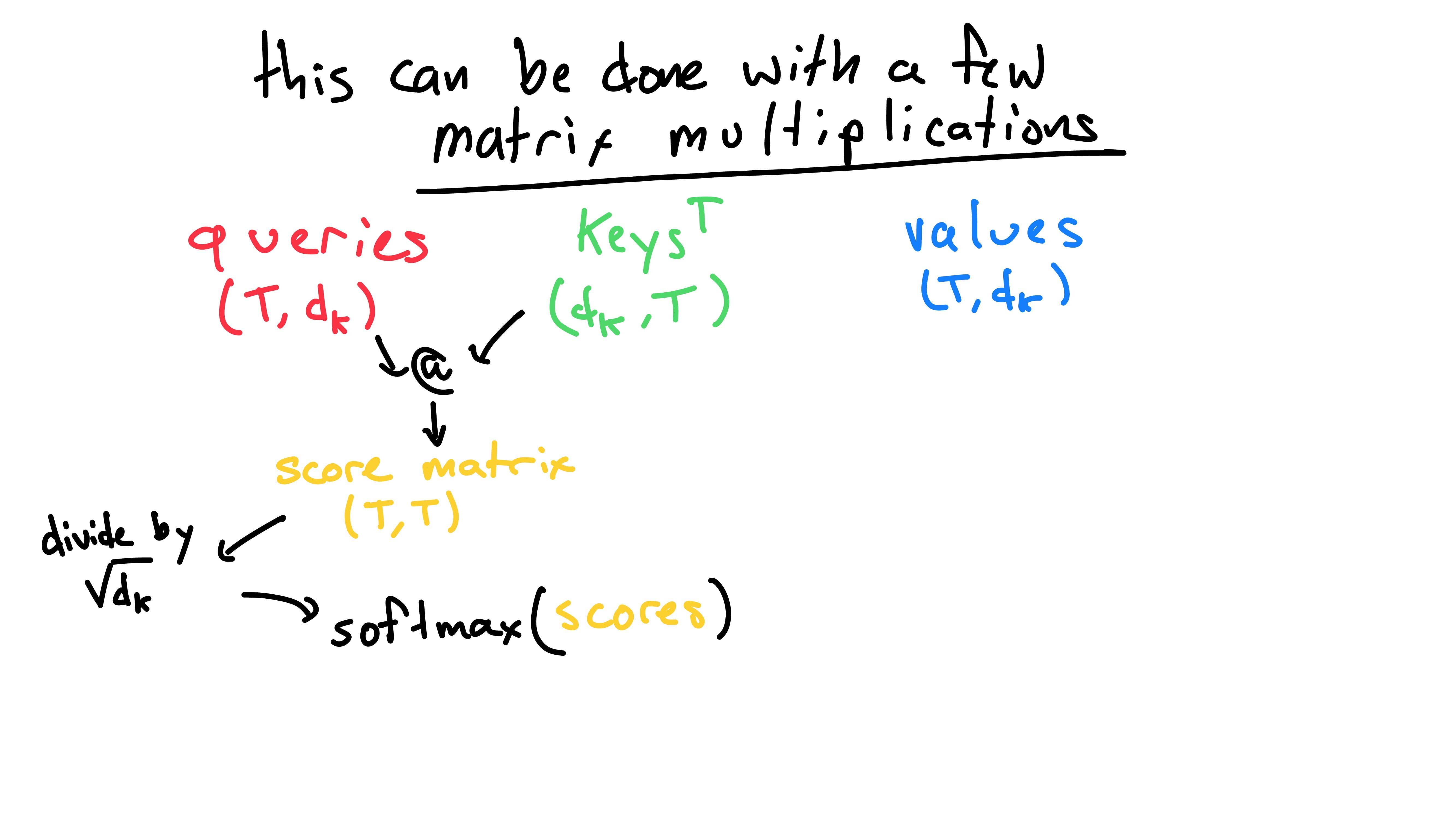
At this point, we need to normalize the scores. There are two steps here:
First, we divide all scores by sqrt(dk). This is done
because the variance of the dot product of two random
vectors (which is what matrix multiplication is composed of)
increases with respect to the length of the vectors. To
counteract this increasing variance, we divide all the scores by the
square of the vector’s length, sqrt(dk). I’ll get to why
we’d want to do this in a moment - for now, onto softmax.
As we recall, the softmax function squishes all values between zero and one, such that the sum of the values adds up to one. We do this so that when we sum up the normalized value vectors, the multiplier adds up to one. Because of this, it wouldn’t make sense to take the softmax of the entire scores matrix once. Instead, we want to take the softmax along the first dimension (one-indexed) - on each row in the matrix (the rows correspond to a singular query and every key). For people who use PyTorch, that’ll look like this:
F.softmax(scores, dim=0)Now that we’ve covered the softmax step, let’s take a step back to
the division by sqrt(dk). (Note: if this reasoning is
unclear, feel free to skip to the next slide.) Some readers might look
at what I wrote and wonder: “Carter, if we’re just going to take the
softmax next anyways, why would we need to scale it? Why do we care
about the variance?” Well, the reason why the variance is important is
because the softmax function has more peaky vs. sparse results when the
variance is greater. Consider the following example:
F.softmax([-1, 0, 1]) = [0.0900, 0.2447, 0.6652]
F.softmax([-10., 0., 10.]) = [2.0611e-09, 4.5398e-05, 9.9995e-01]
F.softmax([-100., 0., 100.]) = [0.0000e+00, 3.7835e-44, 1.0000e+00]
As the variance increases, the results from the softmax function are
more “peaky”, meaning they tend to have one value close to one and
others close to zero (as opposed to all values being more equal). This
is detrimental because it means that the gradient, which is necessary
for gradient-based optimization, “vanishes” to be tiny (bad). This makes
it much more difficult for the network to learn. In other words, the
gradient is “how sensitive the output is to small changes to the input.”
Because the output of the softmax wouldn’t change much, say if
-10 was changed to -9, the network doesn’t
know how to improve.
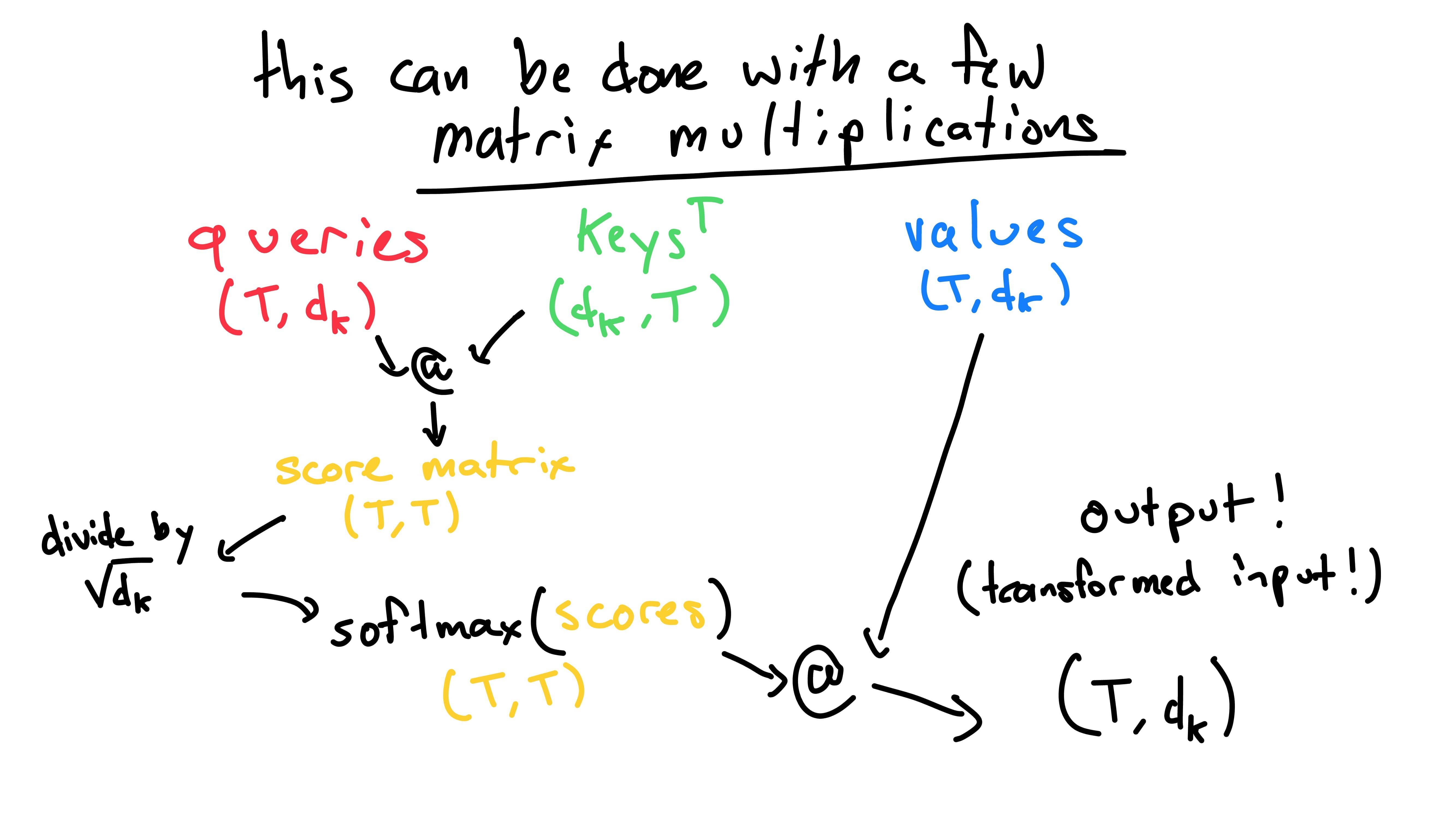
Once we have the softmaxed scores, we can matrix multiply them with
the values. This does the weight values and then sum them in one step,
for all queries. We are then left with our transformed word
matrix of the same shape as the original: (T, dk).
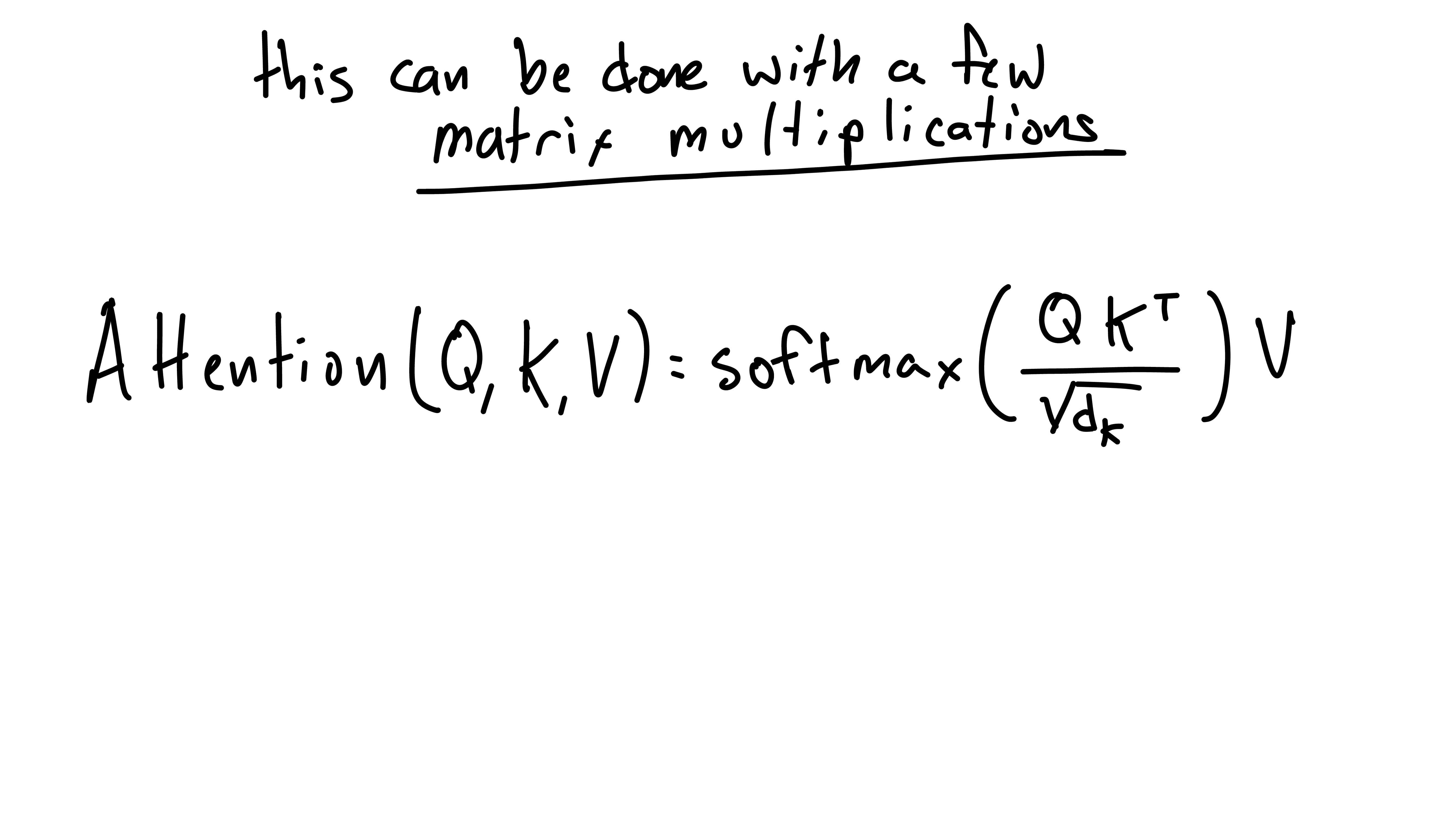
This entire self-attention operation is then neatly represented in the above self-attention formula!
The general idea of multi-headed attention is to allow multiple attention operations over different parts of the vector subspace. This allows GPT to represent different parts of meaning in different ways - allowing greater understanding. Let’s take a look at how this is done:
Previously, our key, value, and query matrices would all be pumped into one attention function.
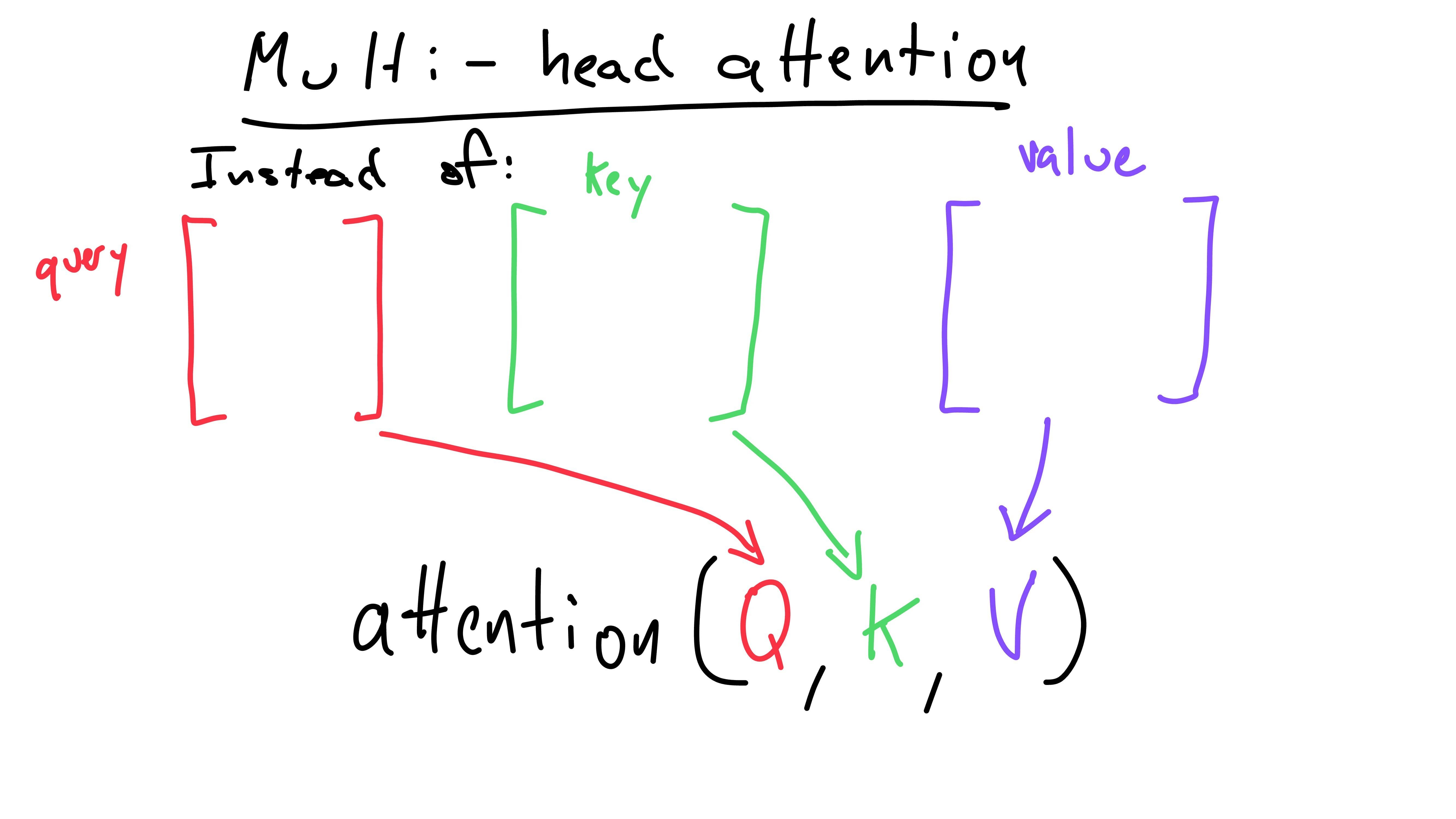
Multi-headed attention instead splits up the query, key, and value
matrices into h number of smaller matrices.
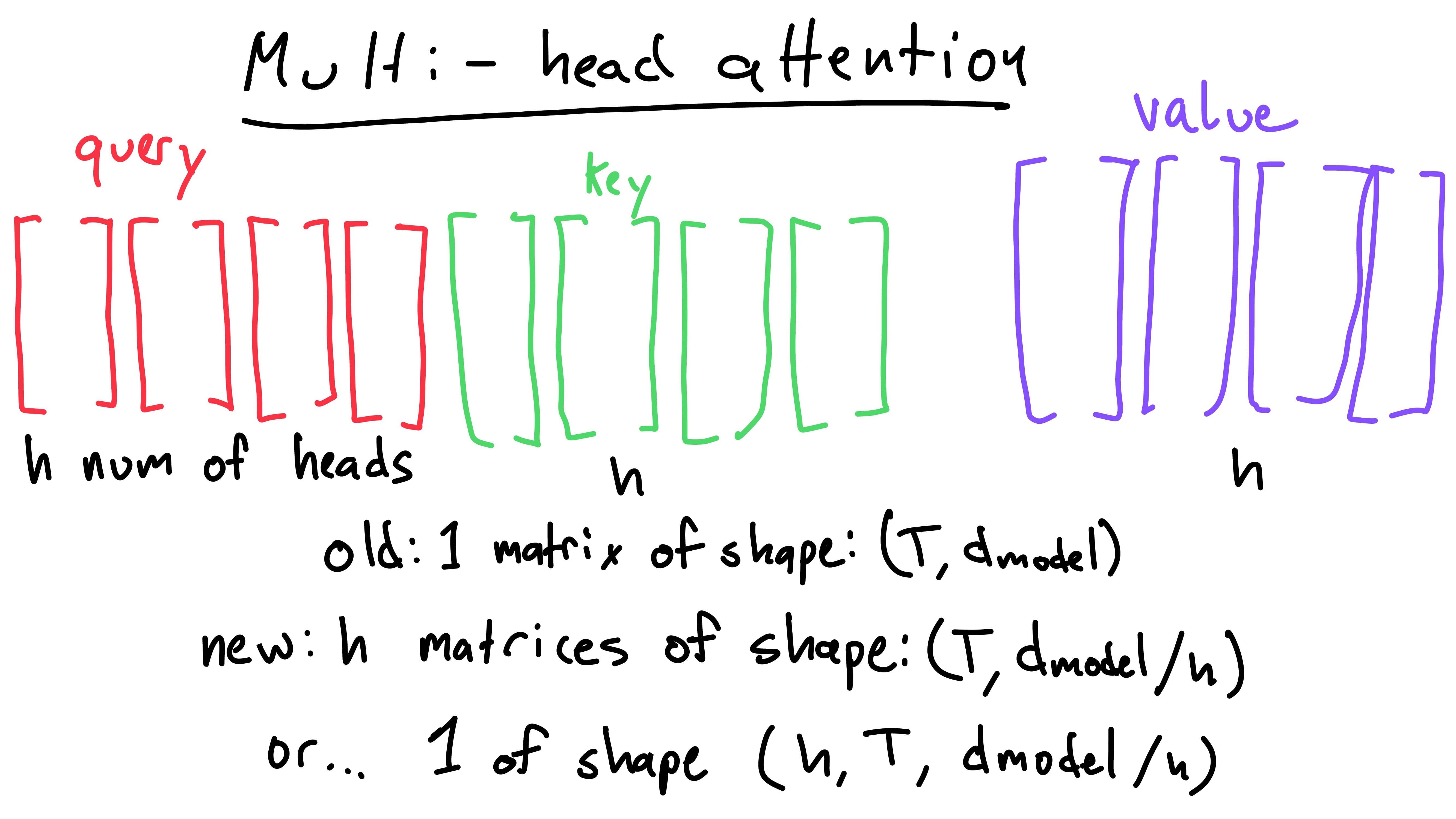
These matrices are split up along the dk dimension, not
the T dimension. This means that each head matrix for the
query, key, or value has shape: (T, d_model / h). Note that
each head still has a row for each word in the sequence, but the second
dimension refers to a smaller part of the word’s subspace.
We now have h key, value, and query matrices. The first
“head” is the group of the first key, value, and query matrix. The
second is the group of the second key, query, and value matrix (and so
on).
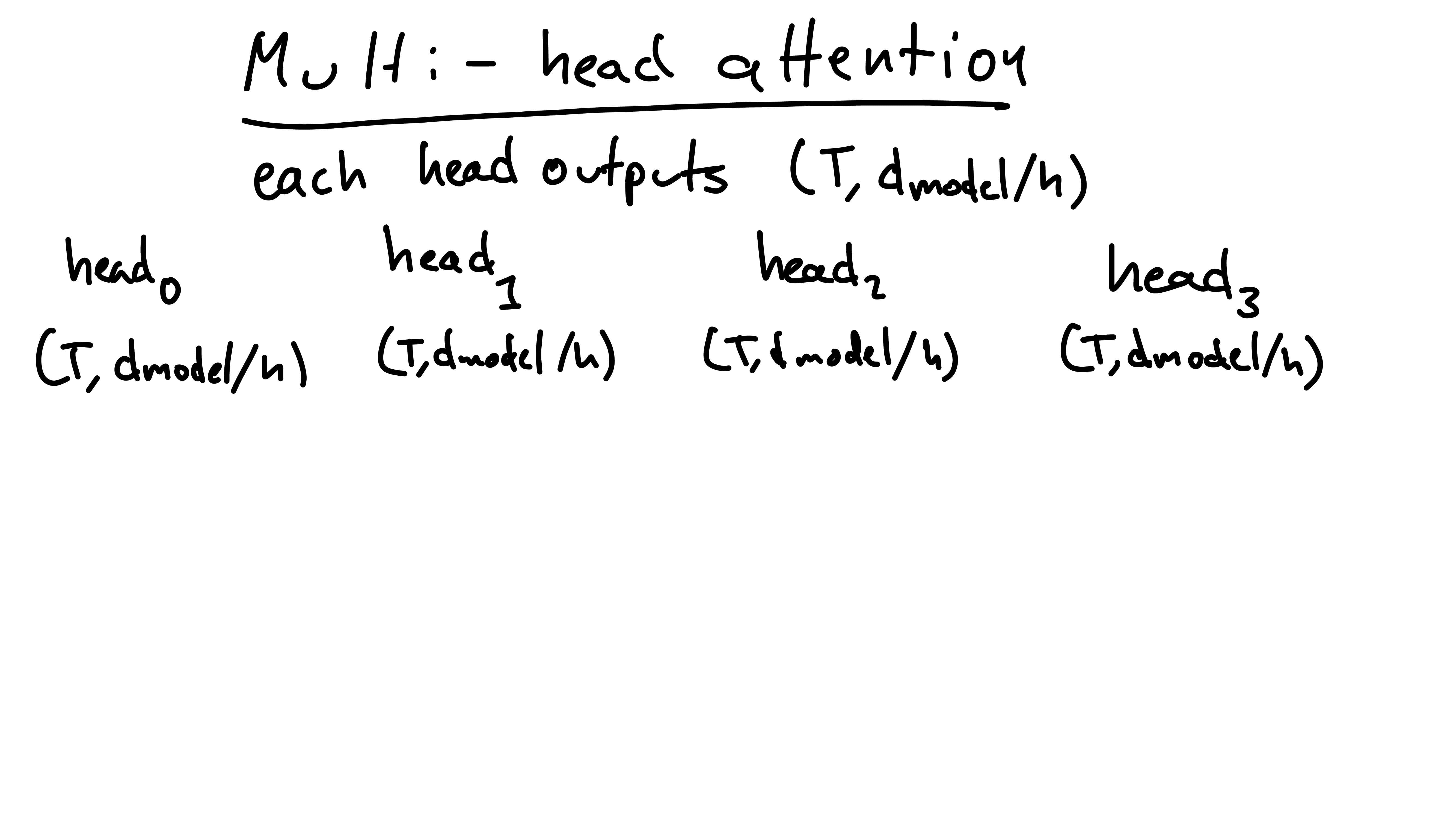
We now conduct self-attention on each head. We do this by running the
key, value, and query matrices for each head through the self-attention
formula we found above. The output shapes for each head are the same
size as the inputs, (T, d_model / h). We now have
h of these head-outputs.
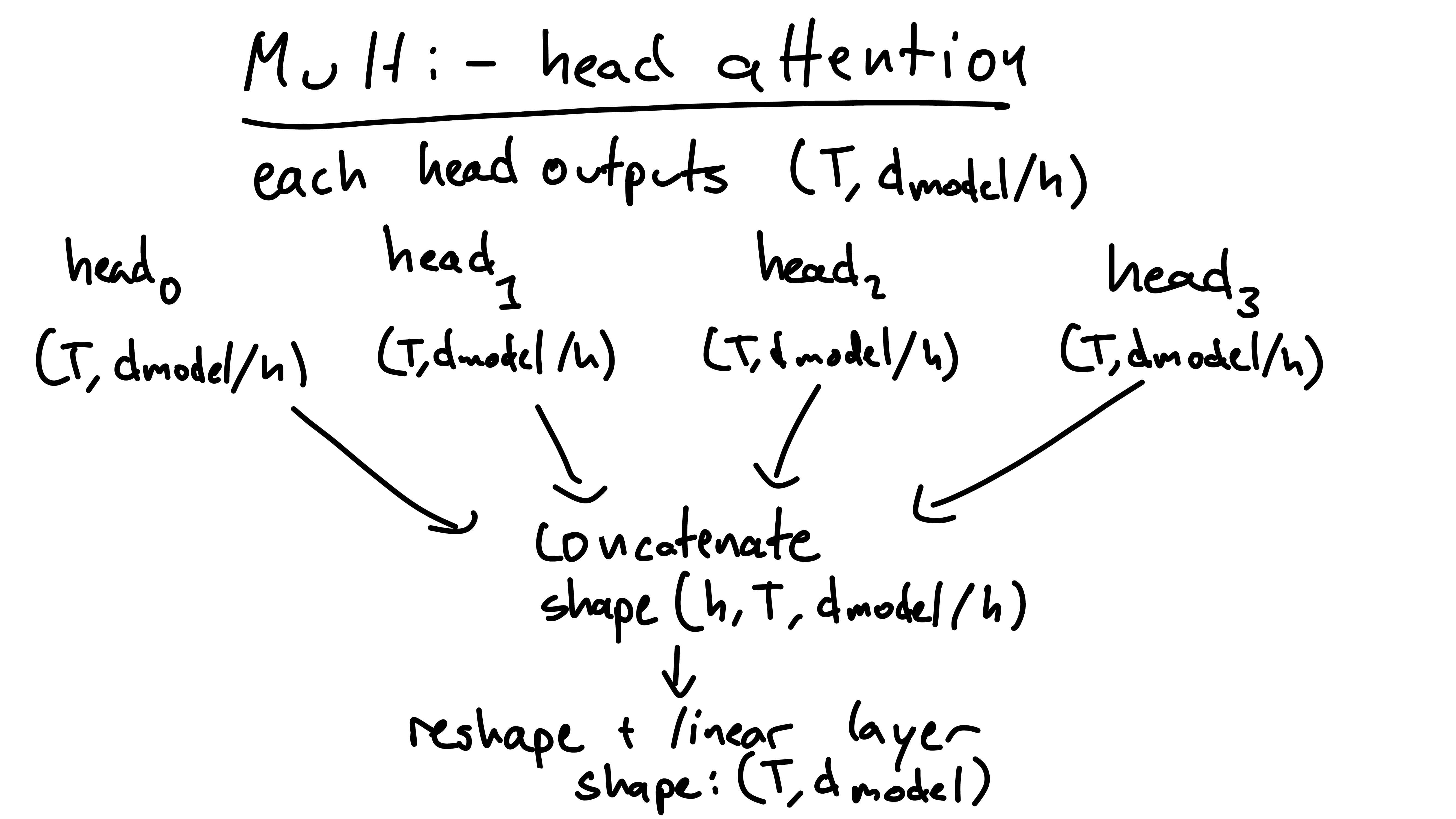
We then concatenate the head outputs into one tensor of shape
(h, T, d_model / h). We reshape this tensor into:
(T, d_model). Finally, we run this through (matrix
multiplication) a linear layer with shape:
(d_model, d_model). This leaves us with out (super!)
transformed output of the input sequence!
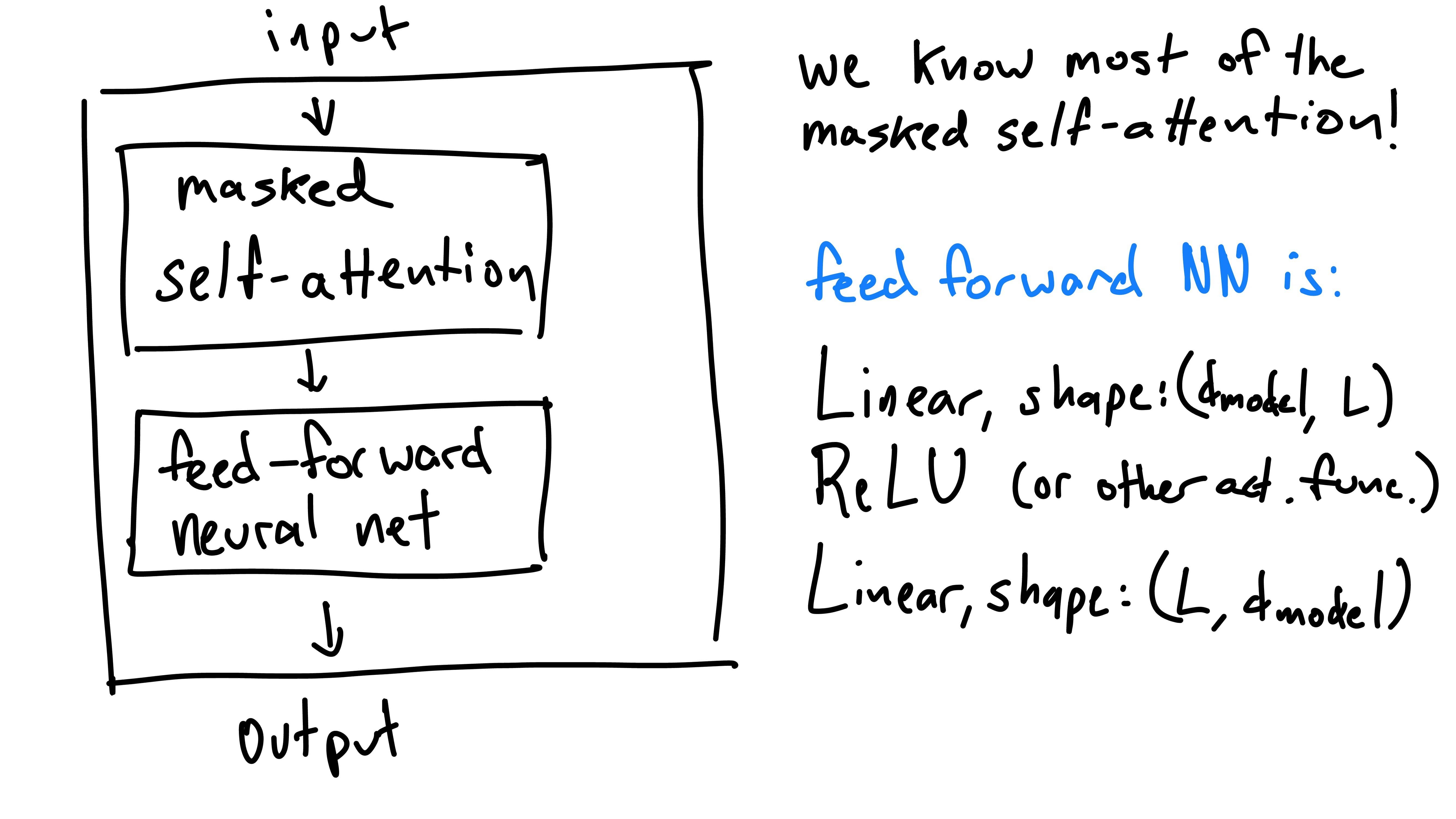
We’re almost done! Now that we have a good idea how masked self-attention works, all that’s left in a decoder block is the feed-forward neural net. This is just two linear layers with a nonlinearity in between (the width of the layers is a hyperparameter one can choose).
This block is what’s repeated throughout GPT - getting this means you’re almost the entire way there to understanding the architecture!
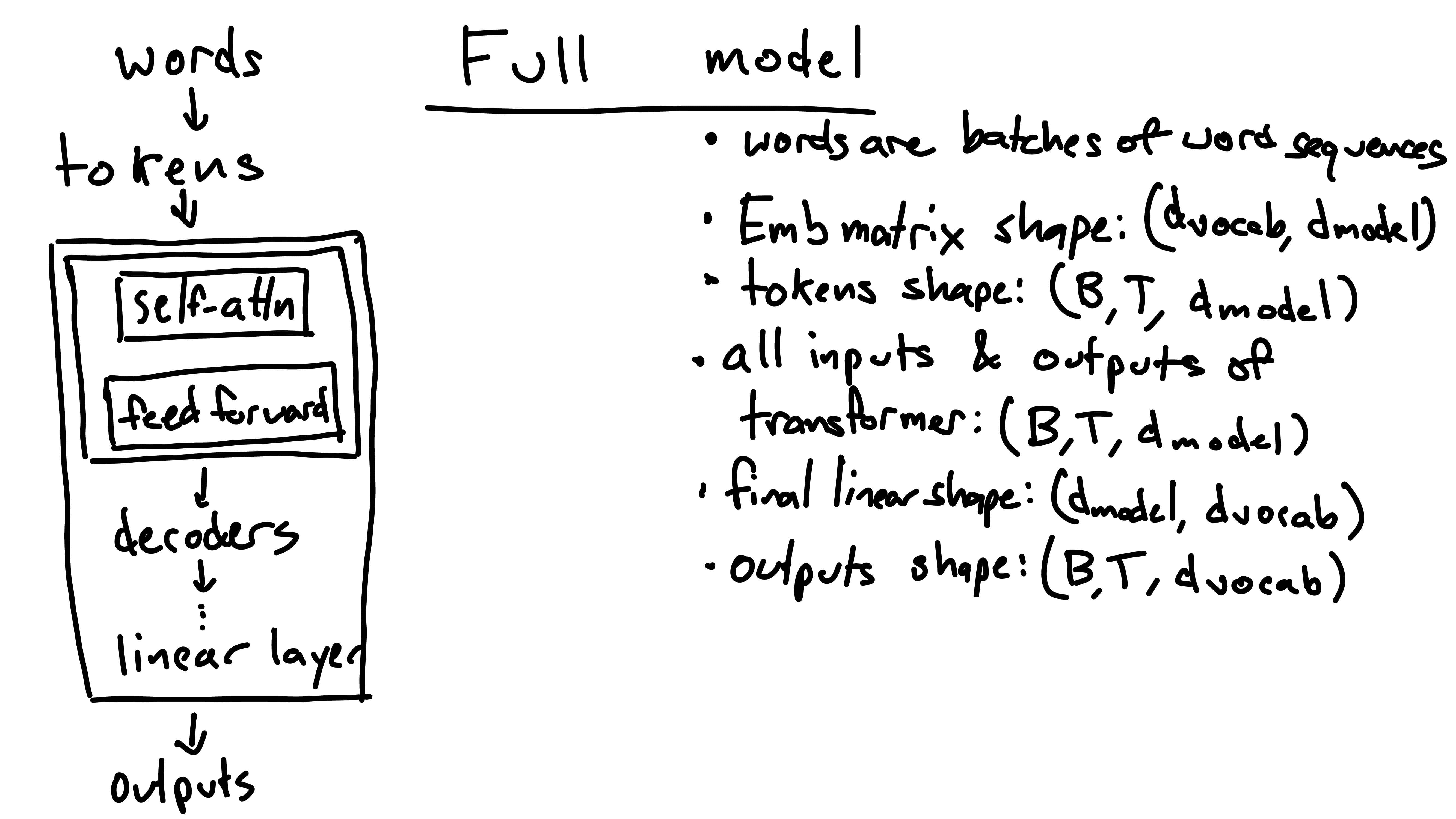
At the end of the model is a linear layer with shape
(d_model, d_vocab). The output (B, T, d_vocab)
of this layer are the unnormalized probabilities of the next token. Each
possible token is given a score for its likelyhood of being next, this
is the d_vocab. Additionally, notice that these next-token
scores are generated for every token in the input. This means that for
every input token, the model predicts the next token - even if the next
token is given in the prompt. For generation we typically only care
about the final input token’s next-token predictions because we care
about predicting tokens we aren’t given.
Here’s a few quick psuedocode examples, given the input sentence:
“The quick brown fox jumps over the lazy dog”. As this is the
only example in the batch, I’ll drop the batch dimension so the output
will be of size: (T, d_vocab).
output = model(tokenized_input) # run the input through the model
print(output[-1])
This should print the vector of length d_vocab
containing the likelyhoods for each word in the vocab being the next
word following the entire input sentence.
print(output[0])
This should print the score vector (similar to above), but for the word following “The”, which is the first word in the input.
print(output[2])
Like the above two examples, this prints the score vector for the word following the input prefix: “The quick brown” - a good model might predict “fox”.
There’s just two finishing points I’d like to make:
Instead of computing the output of each head and then concatenating them, this whole operation can efficiently be done using - you guessed it - matrix multiplication and reshaping. This process is left as an exercise to the reader (or Google it).
I skipped over the “masked” part of masked self-attention. I’ll explain why it’s important and how it works in the next post. If you want to read about it now, I’d recommend The Annotated Transformer.
Thank you for spending your time reading this - I appreciate it! Stay turned for Part 3!
-Carter